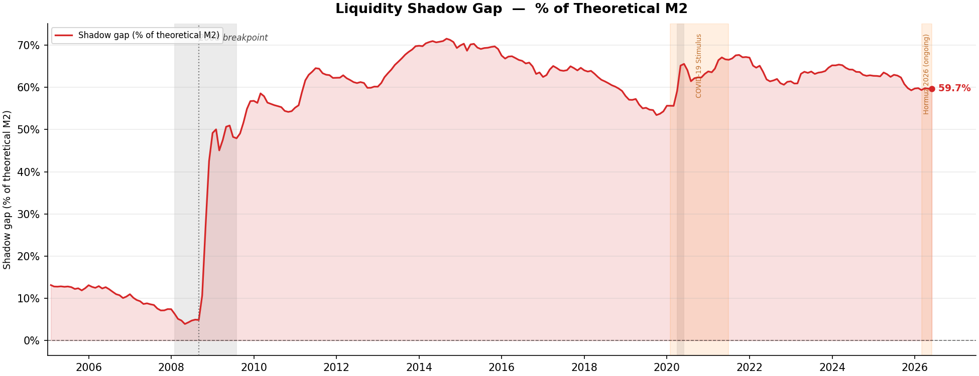
The Liquidity Shadow
A leading indicator buried in the gap between what the money supply is and what it should be — and what happens when you take the second derivative of that gap.
The premise
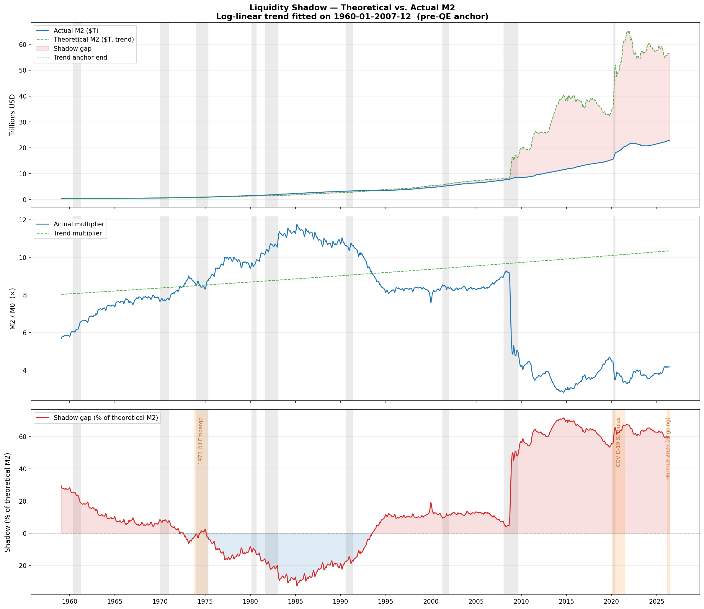
From 1960 through 2007, the money multiplier — the ratio of M2 to the monetary base (M0) — grew along a remarkably stable log-linear trend. Credit markets reliably expanded each Fed dollar into roughly the same multiple of broad money. Banks lent. Multipliers multiplied.
After 2008, that trend broke. The Fed expanded the base massively through quantitative easing, but banks parked the new reserves rather than lending them. The multiplier collapsed. Theoretical M2 — what the money supply would be if the pre-QE trend had continued — diverged sharply from actual M2.
The gap between those two numbers is the liquidity shadow: the credit that should exist under pre-QE mechanics, but doesn't. It's a measure of how far the real economy is operating below its theoretical monetary capacity.
where trend is log-linear fit on 1960–2007 (pre-QE anchor)
Shadow(t) = Theoretical M2(t) − Actual M2(t)
Shadow%(t) = Shadow(t) / Theoretical M2(t) × 100
Shadow% > 0 → actual credit below trend (missing money, stress)
Shadow% < 0 → actual credit above trend (excess liquidity)
The derivative stack
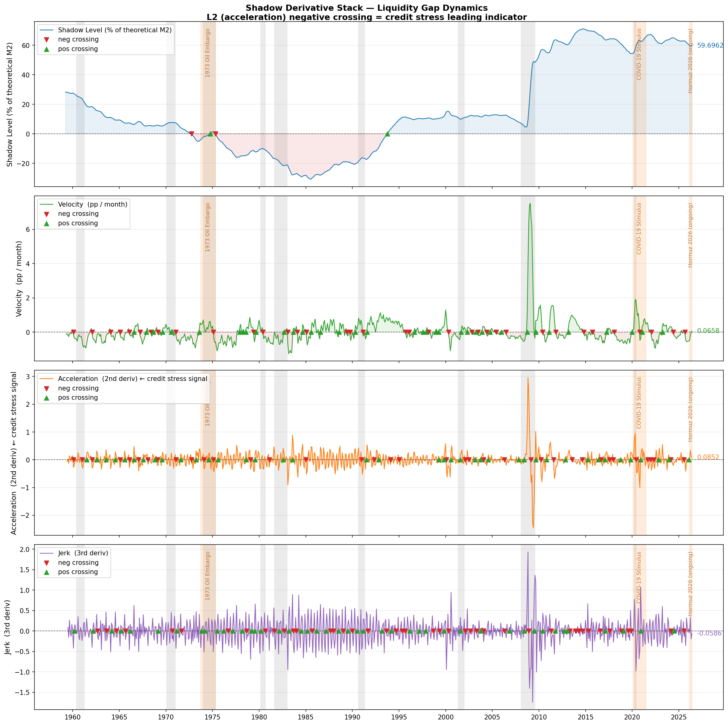
The shadow level alone is useful context. But the rate of change of that gap — and especially the rate of change of the rate of change — is where the predictive signal lives.
The shadow series is smoothed with a rolling mean (to remove month-to-month noise), then differentiated four times in succession:
| Layer | What it measures | Signal interpretation |
|---|---|---|
| L0 | Shadow level (% of theoretical M2) | Gap widening or narrowing overall |
| L1 | Velocity — monthly change in shadow% | Is the gap widening faster or slower? |
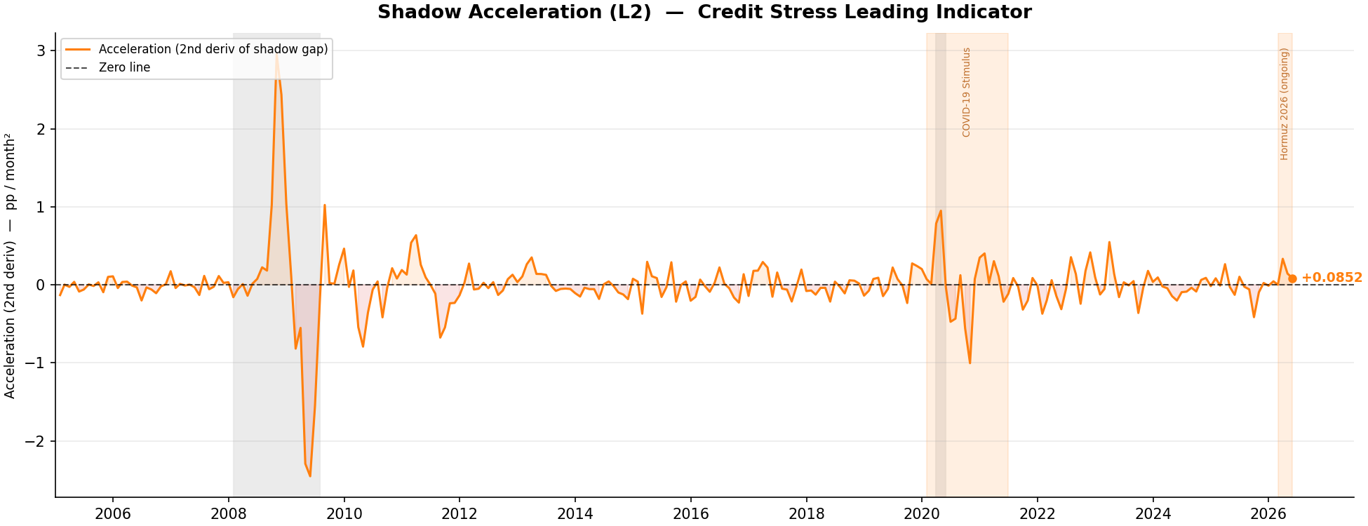
| L2 | Acceleration — 2nd derivative | The leading indicator. Positive = gap accelerating wider (emerging credit stress). Negative crossing = stress decelerating (potential turn). |
| L3 | Jerk — 3rd derivative | Is acceleration itself reversing? Earliest possible warning, highest noise. |
The key finding: L2 zero crossings — where shadow acceleration turns negative after a positive run — have preceded NBER recession starts with measurable and consistent lead times. The signal fires earlier than the level crossing (L0), earlier than velocity (L1), because it catches the turning point of the turning point. By the time the shadow level is obviously widening, the trade is already late.
Breach windows
Beyond individual crossings, the research tracks breach windows: sustained periods (≥3 consecutive months) where L2 is positive — meaning the liquidity gap is not just widening, but widening at an accelerating rate. These windows are the leading edge of credit stress events, and most have mapped within measurable lead times to NBER recession starts.
Exogenous shocks (the 1973 oil embargo, COVID-19 stimulus, the 2026 Hormuz disruption) are flagged separately and excluded from the primary statistics — the signal is designed to detect endogenous credit-cycle stress, not supply-side shocks that fire the indicator for unrelated reasons.
The Cantillon connection
The shadow research runs alongside a parallel indicator: the Cantillon spread — the difference between M2 growth and wage growth. Richard Cantillon observed in 1730 that new money enters the economy at a specific point (then: the royal mint; now: the banking system and primary dealers), and its purchasing power dissipates as it moves outward toward wages and consumer prices.
Cantillon spread = M2 YoY growth − wage YoY growth. A widening spread means asset holders (close to the source) are winning purchasing power faster than workers (at the periphery) can earn it back. A narrowing or inverted spread is a compression signal — often associated with late-cycle conditions or policy reversal.
Combined with the shadow acceleration signal, the Cantillon spread gives a two-axis read: how large is the monetary shortfall, and who is bearing the cost of the transmission gap?